Why is the Closed-Form Solution to Linear Regression Inefficient?
Andrew Carr posted an interesting interview question on Twitter (tweet):
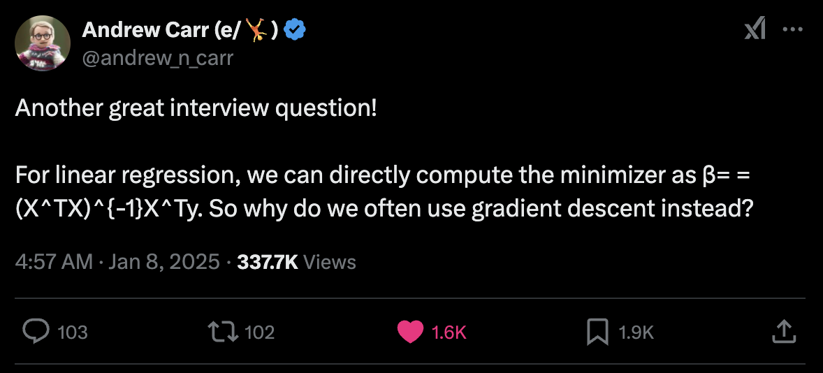
A closed-form solution is a mathematical expression that can be explicitely evaluated using a finite number of standard operations (e.g. addition, multiplication, exponentials, logarithms etc.) without requireing iterative computation. A common example is using the quadratic formula (a closed-form solution) to explicitly evaluate a quadratic equation ax2 + bx + c without iterating over the variables for a, b and c. The closed-form the a linear regression problem is B = (XTX)-1XTy.
Linear regression on the other hand is an iterative solution that iteratively updates the w weights vector to minimise the following cost function J(w):
\[J(w) = \frac{1}{2n} \|Xw - y\|^2\]where:
X = feature matrix
w = coefficients/weights matrix
y = target vector
n = number of samples
It seems naively like if we have an explicit solution that can just be calculated, why bother with this iterative solution? Using the closed-form solution causes two main problems:
- The time-complexity for computing XTX is O(mn2, where m is the number of samples and n is the number of features, and tiem time complexity for computing (XTX)-1 is n3. If your training dataset has many samples or many features, one of these time complexity’s will kill you.
- If X has colinear or nearly colinear features, it is referred to as ill-conditioned, this leads to zero or near-zero eigenvalues which in turn leads to numerical instability when calculating the inversion (XTX)-1 because of the amplification of small floating-point rounding errors, loss of precision, and increased sensitivity to perturbation (small changes in the X dataset, for example with a slightly differently distributed validation set).
For these two reasons, the iterative gradient descent method is preferred for almost all use cases. Gradient descent also always reaches the optimal solution (the local minimum is also the global minimum) if it is properly formulated as it uses a quadratic cost function (mean squared error, MSE) which is a convex function.
To minimise the cost function the algorithm must calculate the gradient of the cost function with respect to each parameter, and then update that parameter based on the learning rate:
\[J(\theta) = \frac{1}{2m} \sum_{i=1}^{m} \left( h_\theta(x^{(i)}) - y^{(i)} \right)^2\] \[\frac{\partial J(\theta)}{\partial \theta_j} = \frac{1}{m} \sum_{i=1}^m \left( h_\theta(x^{(i)}) - y^{(i)} \right) x_j^{(i)}\] \[\theta_j^{(t+1)} = \theta_j^{(t)} - \alpha \frac{\partial J(\theta)}{\partial \theta_j}\]where:
- J(θ): The cost function, which measures the MSE between predictions and actual values.
- m: The number of training examples.
- hθ(x(i)): The predicted value for the i-th example, computed using the hypothesis function, hθ(x) = θθ + θ1x1 + … + θnxn.
- y(i): The true value for the i-th training example.
- ∂J(θ) / ∂θj: Partial derivative of the cost function J(θ) with respect to the parameter θj. This represents how sensitive the cost function is to changes in θj.
- xj(i): The value of the j-th feature for the i-th training example.
- θj(t): The value of the parameter θj at iteration t.
- θj(t+1): The updated value of the parameter θj after the (t+1)-th iteration.
- α: The learning rate, which controls the step size for updating θj. A small α leads to slow convergence, while a large α might cause divergence.
- ∂J(θ) / ∂θj: The gradient of the cost function with respect to θj, which determines the direction and magnitude of the update.